
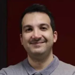
Amir Ghadiri
English and Business Studies Specialist
Gwynedd, United Kingdom
Art and DesignBusiness ManagementBusiness StudiesEnglish Language+3 more
- Currently an Academic Tutor at Bangor University International College (BUIC) and a Visiting Lecturer at Bangor University – Business School (BBS).
- Holds a Master of Science in Computer Science – Creative Arts (Animation & VFX) from University of Dundee (Merit).
- Holds a Bachelor of Arts (Hons) in Linguistics and English Language Studies from the University of Alborz (First Class Honors).
- To progress his Fellowship (FHEA) qualification.
Amir is an english tutor for GCSE–A Level and a business studies tutor for KS2–university and IB; an Academic Tutor at Bangor University International College and Visiting Lecturer at Bangor University Business School, providing session reports and optional homework.
Send a quick enquiry from here and the Latimer Tuition team will pass it on to Amir.